Study Guide - Techniques of Integration

Basic Integration Principles

Integration is the process of finding the region bounded by a function; this process makes use of several important properties.

Learning Objectives

Apply the basic principles of integration to integral problems

Key Takeaways

Key Points

The term integral may also refer to the notion of the anti- derivative, a function $F$ whose derivative is the given function $f$ . In this case, it is called an indefinite integral and is written, $\int f(x)\,dx = F(x) + C$ .
Integration is linear, additive, and preserves inequality of functions.
The definite integral of $f$ over the interval $a$ to $b$ is given by $\int_a^b f = F\vert_a^b$ , where $F$ is an anti-derivative of $f$ .

Key Terms

integration: the operation of finding the region in the x-y plane bound by the function

Integration is an important concept in mathematics and—together with its inverse, differentiation—is one of the two main operations in calculus. Given a function

f

of a real variable

x

, and an interval

[a, b]

of the real line, the definite integral

\int_a^b \! f(x)\,dx

is defined informally to be the area of the region in the

xy

-plane bounded by the graph of

f

, the

x

-axis, and the vertical lines

x=a

and

x=b

, such that area above the

x

-axis adds to the total, and that below the

x

-axis subtracts from the total. The term integral may also refer to the notion of the anti-derivative, a function

F

whose derivative is the given function

f

.

Definite Integral: A definite integral of a function can be represented as the signed area of the region bounded by its graph.

More rigorously, once an anti-derivative

F

of

f

is known for a continuous real-valued function

f

defined on a closed interval

[a, b]

, the definite integral of

f

over that interval is given by

\displaystyle{\int_a^b \! f(x)\,dx = F(b) - F(a)}

If

F

is one anti-derivative of

f

, then all other anti-derivatives will have the form

F(x) + C

for some constant

C

. The collection of all anti-derivatives is called the indefinite integral of

f

and is written as

\displaystyle{\int f\; \mathrm d x = F(x) + C}

Integration proceeds by adding up an infinite number of infinitely small areas. This sum can be computed by using the anti-derivative.

Properties

Linearity

The integral of a linear combination is the linear combination of the integrals.

\displaystyle{\int_a^b (\alpha f + \beta g)(x) \, dx = \alpha \int_a^b f(x) \,dx + \beta \int_a^b g(x) \, dx}

Inequalities

If

f(x) \leq g(x)

for each

x

in

[a, b]

, then each of the upper and lower sums of

f

is bounded above by the upper and lower sums, respectively, of

g

:

\displaystyle{\int_a^b f(x) \, dx \leq \int_a^b g(x) \, dx}

Additivity

If

c

is any element of

[a, b]

, then:

\displaystyle{\int_a^b f(x) \, dx = \int_a^c f(x) \, dx + \int_c^b f(x) \, dx}

Reversing Limits of Integration

If

a > b

,

\displaystyle{\int_a^b f(x) \, dx = - \int_b^a f(x) \, dx}

Integration by Substitution

By reversing the chain rule, we obtain the technique called integration by substitution. Given two functions

f(x)

and

g(x)

, we can use the following identity:

\displaystyle{\int [f'(g(x)) \cdot g'(x)]\; \mathrm d x = f(g(x)) + C}

or written in terms of the "dummy variable"

u = g(x)

:

\displaystyle{\int f'(u)\; \mathrm d u = f(u) + C}

If we are going to use integration by substitution to calculate a definite integral, we must change the upper and lower bounds of integration accordingly.

Integration By Parts

Integration by parts is a way of integrating complex functions by breaking them down into separate parts and integrating them individually.

Learning Objectives

Solve integrals by using integration by parts

Key Takeaways

Key Points

Integration by parts is a theorem that relates the integral of a product of functions to the integral of their derivative and anti-derivative.
The theorem is expressed as $\int u(x) v'(x) \, dx = u(x) v(x) - \int u'(x) v(x) \, dx$ .
Integration by parts may be interpreted graphically in addition to mathematically.

Key Terms

integral: also sometimes called antiderivative; the limit of the sums computed in a process in which the domain of a function is divided into small subsets and a possibly nominal value of the function on each subset is multiplied by the measure of that subset, all these products then being summed
derivative: a measure of how a function changes as its input changes

Introduction

In calculus, integration by parts is a theorem that relates the integral of a product of functions to the integral of their derivative and anti-derivative. It is frequently used to find the anti-derivative of a product of functions into an ideally simpler anti-derivative. The rule can be derived in one line by simply integrating the product rule of differentiation.

Theorem of integration by parts

Let's take the functions

u = u(x)

and

v = v(x)

. When taking their derivatives, we are left with

du = u '(x)

and

dxdv = v'(x) dx

. Now, let's take a look at the principle of integration by parts:

\displaystyle{\int u(x) v'(x) \, dx = u(x) v(x) - \int u'(x) v(x) \ dx}

or, more compactly,

\displaystyle{\int u \, dv=uv-\int v \, du}

Proof

Suppose

u(x)

and

v(x)

are two continuously differentiable functions. The product rule states:

\displaystyle{\frac{d}{dx}\left(u(x)v(x)\right) = u(x) \frac{d}{dx}\left(v(x)\right) + \frac{d}{dx}\left(u(x)\right) v(x)}

Integrating both sides with respect to

x

, over an interval

a \leq x \leq b

,

\displaystyle{\int_a^b \frac{d}{dx}\left(u(x)v(x)\right)\,dx = \int_a^b u'(x)v(x)\,dx + \int_a^b u(x)v'(x)\,dx}

then applying the fundamental theorem of calculus,

\displaystyle{\int_a^b \frac{d}{dx}\left(u(x)v(x)\right)\,dx = \left[u(x)v(x)\right]_a^b}

gives the formula for "integration by parts":

\displaystyle{\left[u(x)v(x)\right]_a^b = \int_a^b u'(x)v(x)\,dx + \int_a^b u(x)v'(x)\,dx}

.

Visulization

Let's define a parametric curve by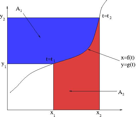

(x, y) = (f(t), g(t))

.

Integration By Parts: Integration by parts may be thought of as deriving the area of the blue region from the total area and that of the red region. The area of the blue region is $A_1=\int_{y_1}^{y_2}x(y)dy$ . Similarly, the area of the red region is $A_2=\int_{x_1}^{x_2}y(x)dx$ . The total area, $A_1+A_2$ _, is equal to the area of the bigger rectangle, $x_2y_2$ , minus the area of the smaller one, $x_1y_1$ : $\int_{y_1}^{y_2}x(y)dy+\int_{x_1}^{x_2}y(x)dx=\biggl.x_iy_i\biggl|_{i=1}^{i=2}$ . Assuming the curve is smooth within a neighborhood, this generalizes to indefinite integrals $\int xdy + \int y dx = xy$ , which can be rearranged to the form of the theorem: $\int xdy = xy - \int y dx$ .

Example

In order to calculate

I=\int x\cos (x) \,dx

, let:

u = x \\ \therefore du = dx

and

dv = \cos(x)\,dx \\ \therefore v = \int\cos(x)\,dx = \sin x

then:

\begin{align} \int x\cos (x) \,dx & = \int u \, dv \\ & = uv - \int v \, du \\ & = x\sin (x) - \int \sin (x) \,dx \\ & = x\sin (x) + \cos (x) + C \end{align}

Trigonometric Integrals

The trigonometric integrals are a specific set of functions used to simplify complex mathematical expressions in order to evaluate them.

Learning Objectives

Solve basic trigonometric integrals

Key Takeaways

Key Points

Some of the expressions for the trigonometric integrals are found using properties of trigonometric functions.
Some of the expressions were derived using techniques like integration by parts.
There is no guarantee that a trigonometric integral has an analytic expression.

Key Terms

trigonometric: relating to the functions used in trigonometry: $\sin$ , $\cos$ , $\tan$ , $\csc$ , $\cot$ , $\sec$
integral: also sometimes called antiderivative; the limit of the sums computed in a process in which the domain of a function is divided into small subsets and a possibly nominal value of the function on each subset is multiplied by the measure of that subset, all these products then being summed

Trigonometric Integrals

The trigonometric integrals are a family of integrals which involve trigonometric functions (

\sin

,

\cos

,

\tan

,

\csc

,

\cot

,

\sec

). The following is a list of integrals of trigonometric functions. Some of them were computed using properties of the trigonometric functions, while others used techniques such as integration by parts. Generally, if the function,

\sin(x)

, is any trigonometric function, and

\cos(x)

is its derivative, then

\displaystyle{\int a\cos nx\;\mathrm{d}x = \frac{a}{n}\sin nx+C}

In all formulas, the constant

a

is assumed to be nonzero, while

C

denotes the integration constant.

Integrands Involving Only Sine:

\displaystyle{\int\sin ax\;\mathrm{d}x = -\frac{1}{a}\cos ax+C\,\! \\ \int\sin^2 {ax}\;\mathrm{d}x = \frac{x}{2} - \frac{1}{4a} \sin 2ax +C= \frac{x}{2} - \frac{1}{2a} \sin ax\cos ax +C\! \\ \int\sin^3 {ax}\;\mathrm{d}x = \frac{\cos 3ax}{12a} - \frac{3 \cos ax}{4a} +C\! \\ \int x\sin^2 {ax}\;\mathrm{d}x = \frac{x^2}{4} - \frac{x}{4a} \sin 2ax - \frac{1}{8a^2} \cos 2ax +C\! \\ \int x^2\sin^2 {ax}\;\mathrm{d}x = \frac{x^3}{6} - \left( \frac {x^2}{4a} - \frac{1}{8a^3} \right) \sin 2ax - \frac{x}{4a^2} \cos 2ax +C\!}

Integrands Involving Only Cosine:

\int\cos ax\;\mathrm{d}x = \frac{1}{a}\sin ax+C

\int\cos^2 {ax}\;\mathrm{d}x = \frac{x}{2} + \frac{1}{4a} \sin 2ax +C = \frac{x}{2} + \frac{1}{2a} \sin ax\cos ax +C

\int\cos^n ax\;\mathrm{d}x = \frac{\cos^{n-1} ax\sin ax}{na} + \frac{n-1}{n}\int\cos^{n-2} ax\;\mathrm{d}x \qquad\mbox{(for }n>0\mbox{)}

\int x\cos ax\;\mathrm{d}x = \frac{\cos ax}{a^2} + \frac{x\sin ax}{a}+C

\int x^2\cos^2 {ax}\;\mathrm{d}x = \frac{x^3}{6} + \left( \frac {x^2}{4a} - \frac{1}{8a^3} \right) \sin 2ax + \frac{x}{4a^2} \cos 2ax +C

Integrands Involving Only Tangent:

\begin{align}\int\tan ax\;\mathrm{d}x &= -\frac{1}{a}\ln \left|\cos ax \right|+C\\ & = \frac{1}{a}\ln \left|\sec ax \right|+C\end{align}

\displaystyle{\int\tan^n ax\;\mathrm{d}x = \frac{1}{a(n-1)}\tan^{n-1} ax-\int\tan^{n-2} ax\;\mathrm{d}x}

where

n \neq 1

; and

\displaystyle{\int\frac{\mathrm{d}x}{q \tan ax + p} = \frac{1}{p^2 + q^2}(px + \frac{q}{a}\ln \left|q\sin ax + p\cos ax \right|)+C }

where

p^2 + q^2 \neq 0

.

Integrands Involving Only Secant:

\displaystyle{\int \sec{ax} \, \mathrm{d}x = \frac{1}{a}\ln{\left| \sec{ax} + \tan{ax}\right|}+C}

\displaystyle{\int \sec^2{x} \, \mathrm{d}x = \tan{x}+C}

Integrands involving only cosecant:

\displaystyle{\int \csc{ax} \, \mathrm{d}x = \frac{1}{a}\ln{\left| \csc{ax}-\cot{ax}\right|}+C}

\displaystyle{\int \csc^2{x} \, \mathrm{d}x = -\cot{x}+C}

Complicated Trigonometric Integrals

We now look at integrals involving the product of a power of

\sin x

and a power of

\cos x

. Two simple examples of such integrals are

\int \sin^k x \cos x \; \mathrm d x

and

\int \cos^k x \sin x\; \mathrm d x

, which can be solved used the substitutions

u = \sin x

and

u = \cos x

, respectively. We now consider the more general case of

\int \sin^n x \cos^m x\; \mathrm d x

, where

n

and

m

are positive integers.

If $n$ is odd, we can pull out one factor of $\sin x$ , convert the rest to cosines using the identity $\sin^2 x + \cos^2 x = 1$ , and then use the substitution $u = \cos x$ .
If $m$ is odd, we can pull out one factor of $\cos x$ , convert the rest to sines using the identity $\sin^2 x + \cos^2 x = 1$ , and then use the substitution $u = \sin x$ .
If both $n$ and $m$ are odd, we can use either of the above two methods.
If both $n$ and $m$ are even, then we can try to use a combination of the following three identities: $\cos^2 x = \frac{1}{2} (1 + \cos 2x)$ , $\sin^2 x = \frac{1}{2} (1 - \sin 2x)$ , and $\sin x \cos x = \frac{1}{2} \sin 2x$ .

Trigonometric Substitution

Trigonometric functions can be substituted for other expressions to change the form of integrands and simplify the integration.

Learning Objectives

Use trigonometric substitution to solve an integral

Key Takeaways

Key Points

If the integrand contains $a^2 − x^2$ , let $x = a \sin(\theta)$ .
If the integrand contains $a^2 + x^2$ , let $x = a \tan(\theta)$ .
If the integrand contains $x^2 - a^2$ , let $x = a \sec(\theta)$ .

Key Terms

trigonometric: relating to the functions used in trigonometry: $\sin$ , $\cos$ , $\tan$ , $\csc$ , $\cot$ , $\sec$

Trigonometric functions can be substituted for other expressions to change the form of integrands. One may use the trigonometric identities to simplify certain integrals containing radical expressions (or expressions containing

n

th roots). The following are general methods of trigonometric substitution, depending on the form of the function to be integrated.

Substitution Rule #1

If the integral contains

a^2-x^2

, let

x = a \sin(\theta)

and use the identity:

1-\sin^2(\theta) = \cos^2(\theta)

Substitution Rule #2

If the integrand contains

a^2+x^2

, let

x = a \tan(\theta)

and use the identity:

1+\tan^2(\theta) = \sec^2(\theta)

Substitution Rule #3

If the integrand contains

x^2-a^2

, let

x = a \sec(\theta)

and use the identity:

\sec^2(\theta)-1 = \tan^2(\theta)

Note that, for a definite integral, one must figure out how the bounds of integration change due to the substitution.

Examples

In order to better understand these substitutions, let's go over the derivation of some of them.

Example 1: Integrals where the integrand contains $a^2 − x^2$ (where $a$ is positive)

In the integral

\displaystyle{\int\frac{dx}{\sqrt{a^2-x^2}}}

we may use:

\displaystyle{x=a\sin(\theta)\\ dx=a\cos(\theta)\,d\theta\\ \theta=\arcsin\left(\frac{x}{a}\right)}

With the substitution, we get:

\begin{align} \int\frac{dx}{\sqrt{a^2-x^2}} & = \int\frac{a\cos(\theta)\,d\theta}{\sqrt{a^2-a^2\sin^2(\theta)}} \\ &= \int\frac{a\cos(\theta)\,d\theta}{\sqrt{a^2(1-\sin^2(\theta))}} \\ &= \int\frac{a\cos(\theta)\,d\theta}{\sqrt{a^2\cos^2(\theta)}} \\ &= \int d\theta \\ &= \theta+C \\ &= \displaystyle{\arcsin \left(\frac{x}{a}\right)}+C \end{align}

Example 2: Integrals where the integrand contains $a^2 − x^2$ (where $a$ is not zero)

In the integral

\displaystyle{\int\frac{dx}{{a^2+x^2}}}

we may use:

\displaystyle{x=a\tan(\theta)\\ dx=a\sec^2(\theta)\,d\theta\\ \theta=\arctan\left(\frac{x}{a}\right)}

With the substitution, we get:

\begin{align}\int\frac{dx}{{a^2+x^2}} &= \int\frac{a\sec^2(\theta)\,d\theta}{{a^2+a^2\tan^2(\theta)}} \\ &= \int\frac{a\sec^2(\theta)\,d\theta}{{a^2(1+\tan^2(\theta))}} \\ &= \int \frac{a\sec^2(\theta)\,d\theta}{{a^2\sec^2(\theta)}} \\ &= \int \frac{d\theta}{a} \\ &= \frac{\theta}{a}+C \\ &= \frac{1}{a} \arctan \left(\frac{x}{a}\right)+C\end{align}

The Method of Partial Fractions

Partial fraction expansions provide an approach to integrating a general rational function.

Learning Objectives

Use partial fraction decomposition to integrate rational functions

Key Takeaways

Key Points

Any rational function of a real variable can be written as the sum of a polynomial and a finite number of rational fractions whose denominator is the power of an irreducible polynomial and whose numerator has a degree lower than the degree of this irreducible polynomial.
The substitution $u = ax + b$ , $du = a \,dx$ reduces the integral as the following: $\int {1 \over ax+b}\,dx = {1 \over a} \ln\left|ax+b\right|+C$ .
When there is an irreducible 2nd-degree polynomial in the denominator, complete the square and change the variable.

Key Terms

irreducible: unable to be factorized into polynomials of lower degree, as $x^2 + 1$

Partial fraction expansions provide an approach to integrating a general rational function. Any rational function of a real variable can be written as the sum of a polynomial and a finite number of rational fractions whose denominator is the power of an irreducible polynomial and whose numerator has a degree lower than the degree of this irreducible polynomial. Here are some common examples.

A 1st-Degree Polynomial in the Denominator

The substitution

u = ax + b

,

du = a \,dx

reduces the integral

\int {1 \over ax+b}\,dx

to:

\begin{align}\int {1 \over u}\,{du \over a}&={1 \over a}\int{du\over u}\\ &={1 \over a}\ln\left|u\right|+C \\ &= {1 \over a} \ln\left|ax+b\right|+C\end{align}

A Repeated 1st-Degree Polynomial in the Denominator

The same substitution reduces such integrals as

\int {1 \over (ax+b)^8}\,dx

to

\begin{align}\int {1 \over u^8}\,{du \over a}&={1 \over a}\int u^{-8}\,du \\ &= {1 \over a} \cdot{u^{-7} \over(-7)}+C \\ &= {-1 \over 7au^7}+C \\ &= {-1 \over 7a(ax+b)^7}+C\end{align}

An Irreducible 2nd-Degree Polynomial in the Denominator

Next we consider integrals such as

\displaystyle{\int {x+6 \over x^2-8x+25}\,dx}

The quickest way to see that the denominator,

x^2 − 8x + 25

, is irreducible is to observe that its discriminant is negative. Alternatively, we can complete the square:

\begin{align}x^2-8x+25&=(x^2-8x+16)+9\\ &=(x-4)^2+9\end{align}

and observe that this sum of two squares can never be

0

while

x

is a real number. In order to make use of the substitution

\begin{align} u & = x^2-8x+25 \\ du & =(2x-8)\,dx \\ \frac{du}{2} & = (x-4)\,dx \end{align}

we would need to find

(x-4)

in the numerator. So we decompose the numerator

x + 6

as

(x-4) + 10

, and we write the integral as

\displaystyle{\int {x-4 \over x^2-8x+25}\,dx + \int {10 \over x^2-8x+25}\,dx}

The substitution handles the first summand, thus:

\begin{align}\int \frac{x-4}{x^2-8x+25}\,dx &= \int \frac{\displaystyle{\frac{du}{2}}}{u} \\ &= \frac{1}{2}\ln\left|u\right|+C \\ &= \frac{1}{2}\ln(x^2-8x+25)+C\end{align}

Note that the reason we can discard the absolute value sign is that, as we observed earlier,

(x-4)^2 + 9

can never be negative. Next we must treat the integral

\displaystyle{\int {10 \over x^2-8x+25} \, dx}

With a little more algebra,

\begin{align} \int {10 \over x^2-8x+25} \, dx &= \int {10 \over (x-4)^2+9} \, dx \\ & = \int \frac{\displaystyle{\frac{10}{9}}}{\left(\displaystyle{\frac{x-4}{3}}\right)^2+1}\,dx \\ &= {10 \over 3} \arctan\left(\frac{x-4}{3}\right) + C \end{align}

Putting it all together:

\displaystyle{\int {x + 6 \over x^2-8x+25}\,dx = {1 \over 2}\ln(x^2-8x+25) + {10 \over 3} \arctan\left({x-4 \over 3}\right) + C}

Integration Using Tables and Computers

Tables of known integrals or computer programs are commonly used for integration.

Learning Objectives

Recognize which integrals should be solved using tables or computers due to their complexity

Key Takeaways

Key Points

While differentiation has easy rules by which the derivative of a complicated function can be found by differentiating its simpler component functions, integration does not.
In books with integral tables, a compilation of a list of integrals and techniques of integral calculus can be found.
There are several commercial softwares, such as Mathematica or Matlab, that can perform symbolic integration.

Key Terms

integral: also sometimes called antiderivative; the limit of the sums computed in a process in which the domain of a function is divided into small subsets and a possibly nominal value of the function on each subset is multiplied by the measure of that subset, all these products then being summed

Integration is the basic operation in integral calculus. While differentiation has easy rules by which the derivative of a complicated function can be found by differentiating its simpler component functions, integration does not, so tables of known integrals are often useful. We also may have to resort to computers to perform an integral.

Integration Using Tables

A compilation of a list of integrals and techniques of integral calculus was published by the German mathematician Meyer Hirsch as early as in 1810. More extensive tables were compiled in 1858 by the Dutch mathematician David de Bierens de Haan. A new edition was published in 1862. These tables, which contain mainly integrals of elementary functions, remained in use until the middle of the 20th century. They were then replaced by the much more extensive tables of Gradshteyn and Ryzhik. Here are a few examples of integrals in these tables for logarithmic functions:

\int\ln ax\;dx = x\ln ax - x

\displaystyle{\int\ln (ax + b)\;dx = \frac{(ax+b)\ln(ax+b) - ax}{a}}

\int (\ln x)^2\; dx = x(\ln x)^2 - 2x\ln x + 2x

\displaystyle{\int (\ln x)^n\; dx = x\sum^{n}_{k=0}(-1)^{n-k} \frac{n!}{k! }(\ln x)^k}

\displaystyle{\int \frac{dx}{\ln x} = \ln\left|\ln x \right| + \ln x + \sum^\infty_{k=2}\frac{(\ln x)^k}{k\cdot k! }}

\displaystyle{\int \frac{dx}{(\ln x)^n} = -\frac{x}{(n-1)(\ln x)^{n-1}} + \frac{1}{n-1}\int\frac{dx}{(\ln x)^{n-1}} \qquad\mbox{(for }n\neq 1\mbox{)}}

You can certainly see that these integrals are hard to do simply "by hand."

Integration Using Computers

Computers may be used for integration in two primary ways. First, numerical methods using computers can be helpful in evaluating a definite integral. There are many methods and algorithms. We will briefly learn about numerical integration in another atom. Second, there are several commercial softwares, such as Mathematica or Matlab, that can perform symbolic integration.

Integration: Numerical integration consists of finding numerical approximations for the value $S$ .

Example: Mathematica's symbolic integration produces the following result:

\int \log(1-x^2) dx = -2x-\log(x-1) + \log(1+x) +x \log(1-x^2).

These programs know how to perform almost any integral that can be done analytically or in terms of standard mathematical functions.

Approximate Integration

The trapezoidal rule (also known as the trapezoid rule or trapezium rule) is a technique for approximating the definite integral

\int_{a}^{b} f(x)\, dx

.

Learning Objectives

Use the trapezoidal rule to approximate the value of a definite integral

Key Takeaways

Key Points

The trapezoidal rule works by approximating the region under the graph of the function $f(x)$ as a trapezoid and calculating its area: $\int_{a}^{b} f(x)\, dx \approx (b-a)\frac{f(a) + f(b)}{2}$ .
For a domain discretized into $N$ equally spaced panels, or $N+1$ grid points $(1, 2, \cdots, N+1)$ , where the grid spacing is $h=\frac{(b-a)}{N}$ , the approximation to the integral becomes $\int_{a}^{b} f(x)\, dx = \frac{b-a}{2N}(f(x_1) + 2f(x_2) + 2f(x_3) + \ldots + 2f(x_N) + f(x_{N+1}))$ .
In two and more dimensions, where simple approximation methods become prohibitively expensive in terms of computational effort, one may use other methods such as the Monte Carlo method.

Key Terms

trapezoid: a (convex) quadrilateral with two (non-adjacent) parallel sides

Numerical integration, in some instances also known as numerical quadrature, asks for the value of a definite integral. Popular methods use one of the Newton–Cotes formulas (such as midpoint rule or Simpson's rule) or Gaussian quadrature. These methods rely on a "divide and conquer" strategy, whereby an integral on a relatively large set is broken down into integrals on smaller sets. In higher dimensions, where these methods become prohibitively expensive in terms of computational effort, one may use other methods such as the Monte Carlo method. Here, we will study a very simple approximation technique, called a trapezoidal rule.

Trapezoidal rule

The trapezoidal rule (also known as the trapezoid rule or trapezium rule) is a technique for approximating the definite integral

\int_{a}^{b} f(x)\,dx

. The trapezoidal rule works by approximating the region under the graph of the function

f(x)

as a trapezoid and calculating its area. It follows that:

\displaystyle{\int_{a}^{b} f(x)\, dx \approx (b-a)\frac{f(a) + f(b)}{2}}

The trapezoidal rule tends to become extremely accurate when periodic functions are integrated over their periods.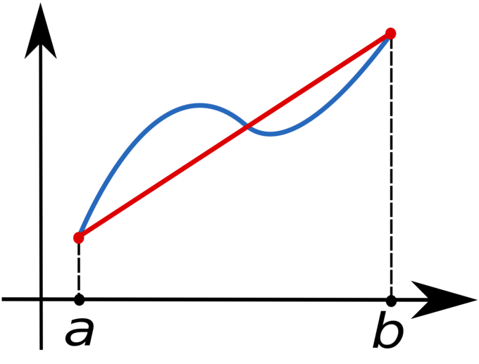

Approximation by Linear Functions: The function $f(x)$ (in blue) is approximated by a linear function (in red).

Numerical Implementation of the Trapezoidal Rule

For a domain discretized into

N

equally spaced panels, or

N+1

grid points

(1, 2, \cdots, N+1)

, where the grid spacing is

h=\frac{(b-a)}{N}

, the approximation to the integral becomes:

\begin{align}\int_{a}^{b} f(x)\, dx &\approx \frac{h}{2} \sum_{k=1}^{N} \left( f(x_{k+1}) + f(x_{k}) \right) {} \\ &= \frac{b-a}{2N}(f(x_1) + 2f(x_2) + \cdots + 2f(x_N) + f(x_{N+1}))\end{align}

Although the method can adopt a nonuniform grid as well, this example used a uniform grid for the the approximation.

Improper Integrals

An Improper integral is the limit of a definite integral as an endpoint of the integral interval approaches either a real number or

\infty

or

-\infty

.

Learning Objectives

Evaluate improper integrals with infinite limits of integration and infinite discontinuity

Key Takeaways

Key Points

An improper integral may be a limit of the form $\lim_{b\to\infty} \int_a^bf(x)\, \mathrm{d}x, \, \lim_{a\to -\infty} \int_a^bf(x)\, \mathrm{d}x$ .
It could also be a limit of the form $\lim_{c\to b^-} \int_a^cf(x)\, \mathrm{d}y,\, \lim_{c\to a^+} \int_c^bf(x)\, \mathrm{d}x$ , in which one takes a limit in one or the other (or sometimes both) endpoints.
It is often necessary to use improper integrals in order to compute a value for integrals which may not exist in the conventional sense (as a Riemann integral, for instance) because of a singularity in the function, or an infinite endpoint of the domain of integration.

Key Terms

integrand: the function that is to be integrated
definite integral: the integral of a function between an upper and lower limit

An improper integral is the limit of a definite integral as an endpoint of the interval(s) of integration approaches either a specified real number or

\infty

or

-\infty

or, in some cases, as both endpoints approach limits. Such an integral is often written symbolically just like a standard definite integral, perhaps with infinity as a limit of integration. But that conceals the limiting process. Specifically, an improper integral is a limit of one of two forms. First, an improper integral could be a limit of the form:

\displaystyle \lim_{b\to\infty} \int_a^bf(x)\, \mathrm{d}x, \, \lim_{a\to -\infty} \int_a^bf(x)\, \mathrm{d}x

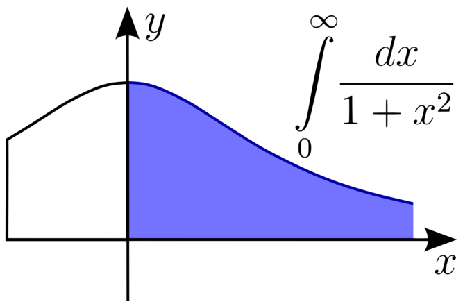
Improper Integral of the First Kind: The integral may need to be defined on an unbounded domain.

Second, an improper integral could be a limit of the form:

\displaystyle \lim_{c\to b^-} \int_a^cf(x)\, \mathrm{d}y,\, \lim_{c\to a^+} \int_c^bf(x)\, \mathrm{d}x

in which one takes a limit at one endpoint or the other (or sometimes both).

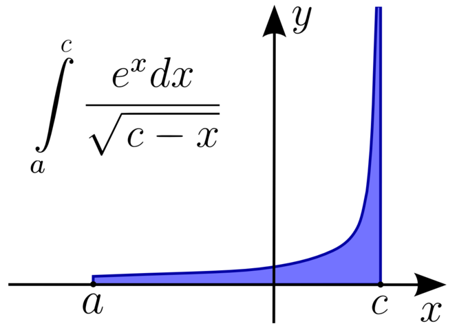
Improper Integral of the Second Kind: An improper Riemann integral of the second kind.The integral may fail to exist because of a vertical asymptote in the function.

Integrals are also improper if the integrand is undefined at an interior point of the domain of integration, or at multiple such points. It is often necessary to use improper integrals in order to compute a value for integrals which may not exist in the conventional sense (as a Riemann integral, for instance) because of a singularity in the function, or an infinite endpoint of the domain of integration.

Example 1

The original definition of the Riemann integral does not apply to a function such as

\frac{1}{x^2}

on the interval

[1, \infty]

, because in this case the domain of integration is unbounded. However, the Riemann integral can often be extended by continuity, by defining the improper integral instead as a limit:

\begin{align} \int_1^\infty \frac{1}{x^2}\,\mathrm{d}x &=\lim_{b\to\infty} \int_1^b\frac{1}{x^2}\,\mathrm{d}x \\ &= \lim_{b\to\infty} \left(-\frac{1}{b} + \frac{1}{1}\right) \\ &= 1\end{align}

Example 2

The narrow definition of the Riemann integral also does not cover the function

\frac{1}{\sqrt{x}}

on the interval

[0, 1]

. The problem here is that the integrand is unbounded in the domain of integration (the definition requires that both the domain of integration and the integrand be bounded). However, the improper integral does exist if understood as the limit

\begin{align}\displaystyle \int_0^1 \frac{1}{\sqrt{x}}\,\mathrm{d}x &=\lim_{a\to 0^+}\int_a^1\frac{1}{\sqrt{x}}\, \mathrm{d}x \\ &= \lim_{a\to 0^+}(2\sqrt{1}-2\sqrt{a})\\ &=2\end{align}

Numerical Integration

Numerical integration constitutes a broad family of algorithms for calculating the numerical value of a definite integral.

Learning Objectives

Solve definite integrals

Key Takeaways

Key Points

The basic problem considered by numerical integration is to compute an approximate solution to a definite integral: $\int_a^b\! f(x)\, dx$ .
There are several reasons for carrying out numerical integration. It could be due to the specific nature of the function (to be integrated) or its antiderivatives.
A large class of quadrature rules can be derived by constructing interpolating functions which are easy to integrate. Typically these interpolating functions are polynomials. Midpoint method and trapezoidal method are simple examples.

Key Terms

trapezoidal: in the shape of a trapezoid, or having some faces which have one pair of parallel sides
antiderivative: an indefinite integral

Numerical integration constitutes a broad family of algorithms for calculating the numerical value of a definite integral, and, by extension, the term is also sometimes used to describe the numerical solution of differential equations. This article focuses on calculation of definite integrals. The term numerical quadrature (often abbreviated to quadrature) is more or less a synonym for numerical integration, especially as applied to one-dimensional integrals. Numerical integration over more than one dimension is sometimes described as cubature, although the meaning of quadrature is understood for higher dimensional integration as well. The basic problem considered by numerical integration is to compute an approximate solution to a definite integral:

\displaystyle{\int_a^b\! f(x)\, dx}

If

f(x)

is a smooth well-behaved function, integrated over a small number of dimensions and the limits of integration are bounded, there are many methods of approximating the integral with arbitrary precision.

Reasons for numerical integration

There are several reasons for carrying out numerical integration. The integrand $f(x)$ may be known only at certain points, such as when obtained by sampling. Some embedded systems and other computer applications may need numerical integration for this reason.
A formula for the integrand may be known, but it may be difficult or impossible to find an antiderivative which is an elementary function. An example of such an integrand $f(x)=\exp(-x^2)$ , the antiderivative of which (the error function, times a constant) cannot be written in elementary form.
It may be possible to find an antiderivative symbolically, but it may be easier to compute a numerical approximation than to compute the antiderivative. That may be the case if the antiderivative is given as an infinite series or product, or if its evaluation requires a special function which is not available.

Methods for One-Dimensional Integrals

A large class of quadrature rules can be derived by constructing interpolating functions which are easy to integrate. Typically these interpolating functions are polynomials. The simplest method of this type is to let the interpolating function be a constant function (a polynomial of degree zero) which passes through the point

\left(\frac{(a+b)}{2}, f\left(\frac{(a+b)}{2}\right)\right)

. This is called the midpoint rule or rectangle rule:

\displaystyle{\int_a^b f(x)\,dx \approx (b-a) \, f\left(\frac{a+b}{2}\right)}

Rectangle Rule: Illustration of the rectangle rule.

The interpolating function may be an affine function (a polynomial of degree 1) which passes through the points

(a, f(a))

and

(b, f(b))

. This is called the trapezoidal rule.

Trapezoidal Rule: Illustration of the trapezoidal rule.

For either one of these rules, we can make a more accurate approximation by breaking up the interval

[a, b]

into some number

n

of subintervals, computing an approximation for each subinterval, then adding up all the results. This is called a composite rule, extended rule, or iterated rule. For example, the composite trapezoidal rule can be stated as

\displaystyle{\int_a^b f(x)\,dx \approx \frac{b-a}{n} \left( {f(a) \over 2} + \sum_{k=1}^{n-1} \left( f \left( a+k \frac{b-a}{n} \right) \right) + {f(b) \over 2} \right)}

where the subintervals have the form

[k h, (k+1) h]

, with

h= \frac{(b-a)}{n}

and

k = 0, 1, 2, \cdots, n−1

.

Study Guides > Boundless Calculus

Techniques of Integration

Basic Integration Principles

Learning Objectives

Key Takeaways

Key Points

Key Terms

Properties

Linearity

Inequalities

Additivity

Reversing Limits of Integration

Integration by Substitution

Integration By Parts

Learning Objectives

Key Takeaways

Key Points

Key Terms

Introduction

Theorem of integration by parts

Proof

Visulization

Example

Trigonometric Integrals

Learning Objectives

Key Takeaways

Key Points

Key Terms

Trigonometric Integrals

Integrands Involving Only Sine:

Integrands Involving Only Cosine:

Integrands Involving Only Tangent:

Integrands Involving Only Secant:

Integrands involving only cosecant:

Complicated Trigonometric Integrals

Trigonometric Substitution

Learning Objectives

Key Takeaways

Key Points

Key Terms

Substitution Rule #1

Substitution Rule #2

Substitution Rule #3

Examples

Example 1: Integrals where the integrand contains a2−x2a^2 − x^2a2−x2 (where aaa is positive)

Example 2: Integrals where the integrand contains a2−x2a^2 − x^2a2−x2 (where aaa is not zero)

The Method of Partial Fractions

Learning Objectives

Key Takeaways

Key Points

Key Terms

A 1st-Degree Polynomial in the Denominator

A Repeated 1st-Degree Polynomial in the Denominator

An Irreducible 2nd-Degree Polynomial in the Denominator

Integration Using Tables and Computers

Learning Objectives

Key Takeaways

Key Points

Key Terms

Integration Using Tables

Integration Using Computers

Approximate Integration

Learning Objectives

Key Takeaways

Key Points

Key Terms

Trapezoidal rule

Numerical Implementation of the Trapezoidal Rule

Improper Integrals

Learning Objectives

Key Takeaways

Key Points

Key Terms

Example 1

Example 2

Numerical Integration

Learning Objectives

Key Takeaways

Key Points

Key Terms

Example 1: Integrals where the integrand contains $a^2 − x^2$ (where $a$ is positive)

Example 2: Integrals where the integrand contains $a^2 − x^2$ (where $a$ is not zero)